Local and Global Shape Estimation

Shape Profiles

Shape profiles depict the ellipsoidal shape of a point cloud as a function of the ellipsoidal radius

\[r_{\text{ell}} = \sqrt{x_{\text{ell}}^2+\frac{y_{\text{ell}}^2}{(b/a)^2}+\frac{z_{\text{ell}}^2}{(c/a)^2}},\]

where \((x_{\text{ell}},y_{\text{ell}},z_{\text{ell}})\) are the coordinates of a point cloud particle in the eigenvector coordinate system of the ellipsoid (= principal frame), i.e., \(r_{\text{ell}}\) corresponds to the semi-major axis \(a\) of the ellipsoidal surface on which that particle lies.

The shape as a function of ellipsoidal radius can be described by the axis ratios

\[q = \frac{b}{r_{\text{ell}}}, \ \ s = \frac{c}{r_{\text{ell}}},\]

where \(b\) and \(c\) are the eigenvalues corresponding to the intermediate and minor axes, respectively. The ratio of the minor-to-major axis \(s\) has traditionally been used as a canonical measure of the distribution’s sphericity. A frequently quoted shape parameter is the triaxiality

\[T = \frac{1-q^2}{1-s^2},\]

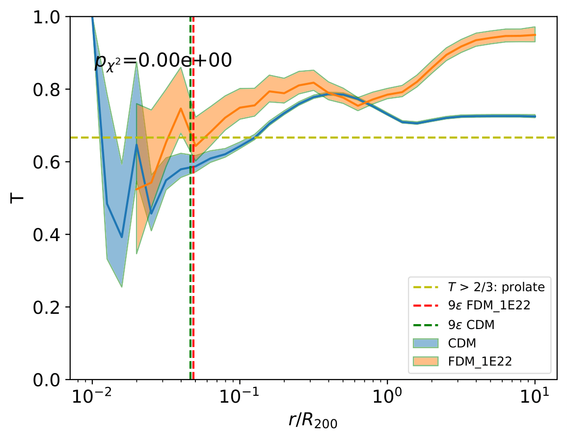
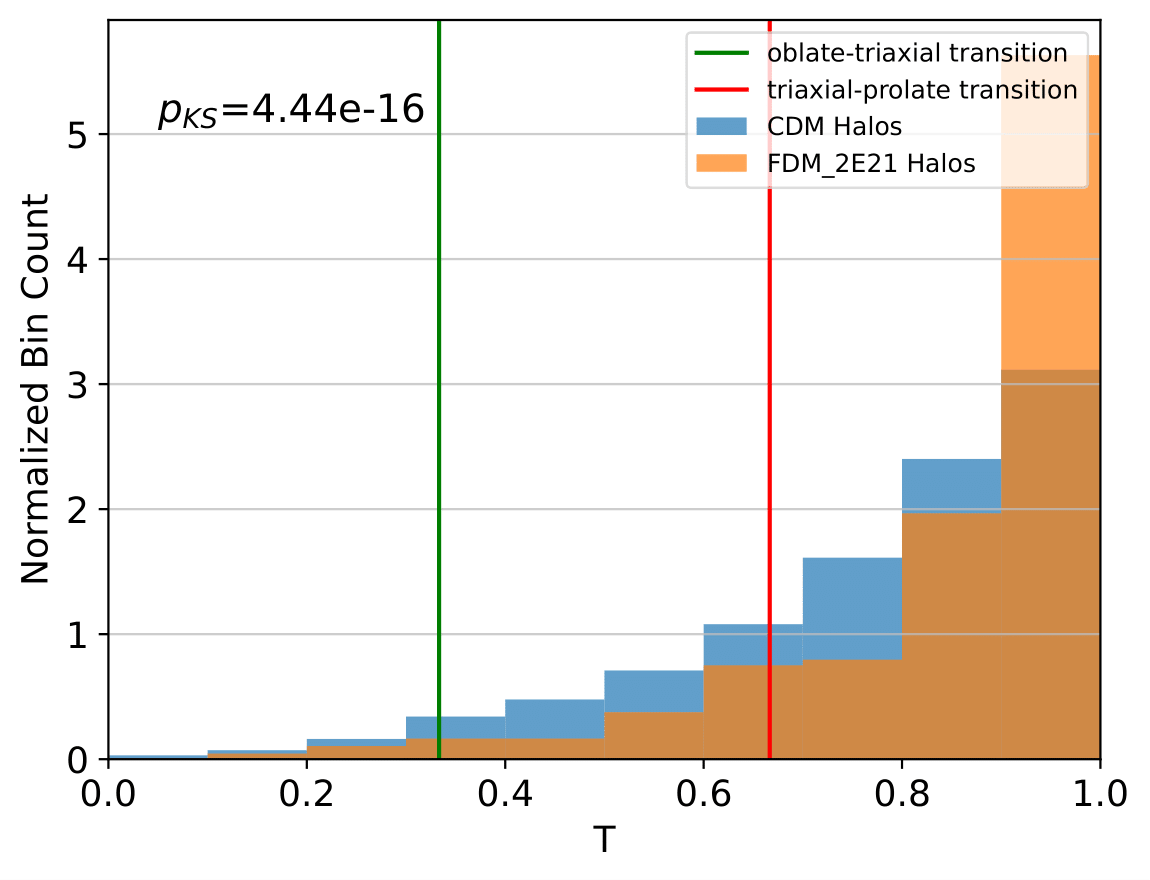
which measures the prolateness/oblateness of a halo. \(T = 1\) describes a completely prolate halo, while \(T = 0\) describes a completely oblate halo. Halos with \(0.33 < T < 0.67\) are said to be triaxial. The axis ratios can be computed from the shape tensor \(S_{ij}\), which is the second moment of the mass distribution divided by the total mass:

\[S_{ij} = \frac{1}{\sum_k m_k} \sum_k w_k m_k r_{k,i}r_{k,j}.\]

Here, \(m_k\) is the mass of the \(k\)-th particle, and \(r_{k} = (x_{k},y_{k},z_{k})^t\) is the position vector with respect to the distribution’s center (either mode or center of mass). The weight \(w_k\) allows to define the most common shape tensors by choosing

\(w_k = 1\), in which case each particle gets the same weight, or
\(w_k = \frac{1}{r_k^2}\) where \(r_k^2 = (x_{k})^2+(y_{k})^2+(z_{k})^2\) is the distance squared of particle \(k\) from the center of the cloud, or
\(w_k = \frac{1}{r_{\text{ell},k}^2}\) where \(r_{\text{ell},k}^2 = x_{\text{ell},k}^2+y_{\text{ell},k}^2+z_{\text{ell},k}^2\) is the ellipsoidal radius, where \((x_{\text{ell},k}, y_{\text{ell},k}, z_{\text{ell},k})\) are the coordinates of particle \(k\) in the eigenvector coordinate system of the ellipsoid. The shape tensor with \(w_k = \frac{1}{r_{\text{ell},k}^2}\) is also called the reduced shape tensor, a variant that penalizes particles at large radii.

Since the second weighting scheme with \(w_k = \frac{1}{r_k^2}\) has fallen out of favour, see Zemp et al. 2011, the other two schemes will be available by switching the boolean REDUCED, see below.

After instantiating an object cprofiles as outlined in Data Structures section, one can calculate and retrieve the local (i.e. as a function of \(r_{\text{ell}}\)) halo shape catalogue by:

shapes = cprofiles.getShapeCatLocal(obj_numbers, katz_config = default_katz_config).

The morphological information in the structured numpy array shapes can be retrieved by dictionary-like semantics. d = shapes['d'], q = shapes['q'], s = shapes['s'], minor = shapes['minor'], inter = shapes['inter'] and major = shapes['major'] represents the shape profiles. The obj_numbers argument expects a list of integers indicating for which objects to estimate the density profile. If e.g. obj_numbers = np.arange(10), only the first 10 objects that have sufficient resolution will be considered. Typically, the ordering of objects internally is such that this will select the 10 most massive objects. CosmicProfiles uses the iterative Katz 1991 algorithm to calculate the shape profiles. The default configuration parameters are:

default_katz_config = {'ROverR200': np.logspace(-1.5,0,70), 'IT_TOL': 1e-2, 'IT_WALL': 100, 'IT_MIN': 10, 'REDUCED': False, 'SHELL_BASED': False},

where ROverR200 contains the normalized ellipsoidal radii of interest, in units of R200 or Rvir (depending on RVIR_OR_R200) of parent halo, at which the shape profiles should be calculated. The float IT_TOL is the convergence tolerance in the shape estimation algorithm: eigenvalue fractions must differ by less than IT_TOL for the algorithm to halt. The integer IT_WALL is the maximum permissible number of iterations in shape estimation algorithm. The integer IT_MIN is the minimum number of particles (DM, gas or star particles depending on OBJ_TYPE) in any iteration. If undercut, the shape remains unclassified (NaNs). The boolean REDUCED allows to select between the reduced shape tensor with weight \(w_k = \frac{1}{r_{\text{ell},k}^2}\) and the regular shape tensor with \(w_k = 1\). The boolean SHELL_BASED allows to run the iterative shape identifier on ellipsoidal shells (= homoeoids) rather than ellipsoids. Note that SHELL_BASED = True should only be set if the number of particles resolving the objects is \(> \mathcal{O}(10^5)\). The dictionary default_katz_config can be imported via from cosmic_profiles import default_katz_config.

Warning

The arrays d, q, s, minor, inter and major that can be retrieved from the structured numpy array shapes will contain NaNs whenever the shape determination does not converge.

Note

We consider the shape determination at a specific \(r_{\text{ell}}\) to be converged if the fractional difference between consecutive eigenvalue fractions falls below IT_TOL and the maximum number of iterations IT_WALL is not yet achieved.

The shapes structured array contains a field is_conv which is True whenever the shape calculation converged, True otherwise. If you wanted to do some analysis on the e.g. 21st halo but wanted to remove unconverged bins, one could do something like:

shape = shapes[20]
is_conv = shapes[20]['is_conv']
shape = shape[is_conv]
...

If \(N_{\text{pass}}\) stands for the number of objects that have been selected with the obj_numbers argument and in addition are sufficiently resolved, then the 1D and 2D shape profile arrays will have the following format:

d of shape (\(N_{\text{pass}}\), D_BINS + 1): ellipsoidal radii
q of shape (\(N_{\text{pass}}\), D_BINS + 1): q shape parameter
s of shape (\(N_{\text{pass}}\), D_BINS + 1): s shape parameter
minor of shape (\(N_{\text{pass}}\), D_BINS + 1, 3): minor axes vs \(r_{\text{ell}}\)
inter of shape (\(N_{\text{pass}}\), D_BINS + 1, 3): intermediate axes vs \(r_{\text{ell}}\)
major of shape (\(N_{\text{pass}}\), D_BINS + 1, 3): major axes vs \(r_{\text{ell}}\)
obj_centers of shape (\(N_{\text{pass}}\),3): centers of objects
obj_masses of shape (\(N_{\text{pass}}\),): masses of objects.

For post-processing purposes, one can dump the shape profiles via:

cprofiles.dumpShapeCatLocal(obj_numbers, katz_config = default_katz_config),

which will save the shape profiles in a destination of choice self.CAT_DEST (a string describing the absolute (or relative with respect to Python working diretory) path to the destination folder, e.g. /path/to/cat, will be created if missing) that has been provided during object instantiation.

Note

In case of a Gadget-style I, II or HDF5 snapshot output, specify OBJ_TYPE = 'dm' to calculate local dark matter halo shapes (only the dark matter component of halos), OBJ_TYPE = 'gas' to calculate the local shapes of gas particles inside halos and OBJ_TYPE = 'stars' to calculate the local shapes of star particles inside halos. The suffix of the output files will be modified accordingly to e.g. d_local_gas_x.txt.

Global Shapes

Instead of shape profiles one might also be interested in obtaining the shape parameters and principal axes of the point clouds as a whole. This information can be obtained by calling:

shapes = cprofiles.getShapeCatGlobal(obj_numbers, katz_config = default_katz_config).

If a global shape calculations does not converge (which is rare), the corresponding entry in q = shapes['q'] etc. will feature a NaN. As with shape profiles, we can dump the global shape catalogue in a destination self.CAT_DEST of choice via:

cprofiles.dumpShapeCatGlobal(obj_numbers, katz_config = default_katz_config),

which will save some files in the destination folder.

Note

As previously, \(N_{\text{pass}}\) denotes the number of halos that have been selected with the obj_numbers argument and pass the MIN_NUMBER_PTCS-threshold. If the global shape determination for a sufficiently resolved object does not converge, it will appear as NaNs in the output.

Velocity Dispersion Tensor Eigenaxes

For Gadget-style I, II, or HDF5 snapshot outputs one can calculate the velocity dispersion tensor eigenaxes by calling:

shapes = cprofiles.getShapeCatVelLocal(obj_numbers, katz_config = default_katz_config)

for local velocity shapes or cprofiles.getShapeCatVelGlobal(obj_numbers, katz_config = default_katz_config) for global velocity shapes. When calling e.g. cprofiles.dumpShapeCatVelGlobal(obj_numbers, katz_config = default_katz_config), the overall halo velocity dispersion tensor shapes of the following format will be added to self.CAT_DEST.

The cprofiles.dumpShapeCatVelLocal(obj_numbers, katz_config = default_katz_config) command will dump files named d_local_vdm_x.txt etc.

Visualizations

Shape profiles can be visualized using:

cprofiles.plotShapeProfs(nb_bins = 2, obj_numbers, katz_config = default_katz_config)

which draws median shape profiles and also mass bin-decomposed ones. nb_bins stand for the number of mass bins to plot density profiles for. 3D visualizations of individual halos can be accomplished using:

cprofiles.vizLocalShapes(obj_numbers = [0,1,2], katz_config = default_katz_config)

which for instance would visualize the 3D distribution of particles as well as the eigenaxes at two different ellipsoidal radii in the first three objects that have sufficient resolution. The shape visualizations will be saved to the object’s attribute self.VIZ_DEST (string describing the absolute (or relative with respect to Python working diretory) path to the visualization folder, e.g. /path/to/viz, will be created if missing) that has been provided during object instantiation.